Special issue statement. This article is part of a special issue published on the occasion of the 70th anniversary of E&G Quaternary Science Journal (EGQSJ). The special issue celebrates the journal's notable contribution to Quaternary research by revisiting selected milestone articles published in the long history of EGQSJ. The German Quaternary Association (DEUQUA) presents translations of the originals and critical appraisals of their impact in tandem anniversary issues of DEUQUASP and EGQSJ, respectively.

Original article: https://doi.org/10.3285/eg.02.1.02

Tribute: https://doi.org/10.5194/egqsj-70-205-2021

Translators: Clare Bamford, Markus Fuchs and Henrik Rother

About 80 of the 100 years that modern scientific research into the Ice Age looks back on today were devoted primarily to the study of the enormous increase in the size of glaciers at that time and the consequences of this phenomenon. In reality, however, the growth of the glaciers is only one – albeit a geomorphologically particularly striking – effect of the ice age climate among many others. In the areas close to the inland ice, a whole series of other exogenous-dynamic effects of the glacial climate have been investigated in more detail in the last two decades, which in their pedological, morphological and stratigraphic effects, spatially and quantitatively exceeded those of the increased glaciers many times over (cf. Büdel, 1944). In addition, the climatic change that occurred eight times during the Pleistocene (at the beginning and end of each glacial period) affected not only the glacier zone and its surroundings (the so-called “periglacial” area), but the whole earth. In brief, this process can be represented in such a way that during the glacial periods the entire climate belt of the earth experienced a shift from the poles to the equator, as shown in Fig. 1 for the northern hemispheric meridian field located between 0 and 15^∘ east.

However, this shift of the atmospheric circulation areas did not only result in a change in latitude qualitatively similar to today's climate zones. In other latitudes, the belts of related circulation were in any case also in a different radiation climate than today. Some of them also had a different latitudinal extension and the new parts of the mainland they took possession of had a different position in relation to the (differently shaped) sea surfaces than today. From the outset, therefore, it must seem impossible to attempt an exhaustive description of the Ice Age climate in its relationship to the present climate by means of the change in a single climatic element or even a single figure (such as a reduction in the mean annual temperature by 7 or 8 ^∘C). Instead, we arrive at the picture of diverse ice age climate zones that differ from today's, each of which can only be characterised by a whole complex of climate values. In order to grasp these complexes, all possible glacial climate traces must be used together, complementing each other. The following individual description refers first of all to ice-age Europe and its neighbouring areas, since the best documents for such an investigation are available here (cf. Büdel, 1949).

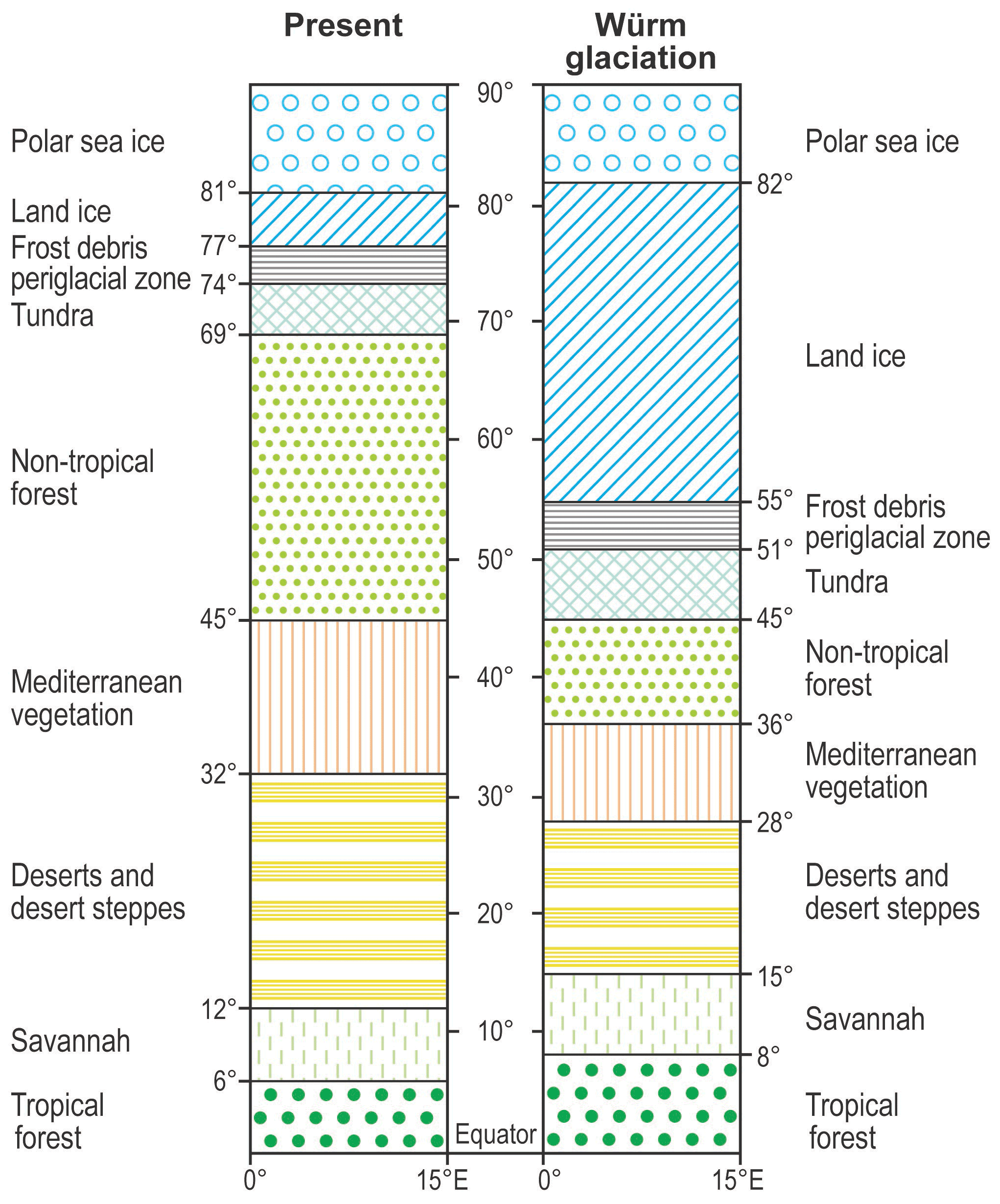
Figure 1Shift of the terrestrial climate zones during the Würm glaciation. The mean latitude of these zones is shown in the meridian field between 0 and 15^∘ east longitude. Apart from the polar sea, the marine areas are assigned to the neighbouring continental climate belts.

Download

For the area described, my student M. Brusch (1949) drew up maps of equal snowline elevations (isochions) on the basis of all accessible material, both for the present and for the Würm glaciation. She found that today's isochions with their general course from WSW to ENE through Europe show a very far-reaching correlation with the (reduced) July isotherms of the present. For example, the 2000 m isochion parallels the 17–18^∘ July isotherm, the 1500 m isochion parallels the 14^∘ July isotherm, and the 1000 m isochion of the present, which runs from Iceland via the Lofoten Islands and the coastal fringe of Finnmarken along the northern edge of Europe to the northern Urals, parallels the 10–11^∘ July isotherm (which, as is well known, largely coincides with the polar tree line). Since this parallelism extends evenly from the oceanic west to the continental east of the continent, I concluded from this that during the ice ages (despite a somewhat different distribution of precipitation at that time) the ice-age July isotherms must basically also have corresponded to the isochions of that time! If the 2000 m isochion is followed by the 17^∘ July isotherm, the 1500 m isochion by the 14^∘ July isotherm, etc., a map of the ice-age July isotherms (reduced to today's sea level) is obtained for the whole area under consideration. The +10.5^∘ July isotherm is again of particular interest to us as a reference point for the course of the polar tree line at that time. It enters the west coast of Europe just south of the mouth of the Gironde in the “Landes” and then runs along the northern edge of the French central plateau and the Jura over the Vosges to the northern Black Forest and on to the northwest of the Harz, where it then runs across the eastern German-Eastern European lowlands in an east-northeast direction to the Mid Urals.

From this line, with the help of orography and the mean reduction factor of 0.5^∘ for 100 m, one can now reconstruct with a fair degree of accuracy the real ice-age July isotherm of +10.5^∘ (drawn in Fig. 2 in France as a thick dotted line, and further eastwards, where it almost completely coincides with the true tree line, as a thick drawn line). On the Atlantic coast, of course, this line also starts from the mouth of the Gironde, but then on French soil it runs around the southern edge of the central plateau and in the Rhone valley it penetrates northwards at the most into the area of Lyon. At the same time, this isotherm encloses the Pyrenees and the other mountains of the Iberian Peninsula in an isolated course. In a similar way, this line also extends far to the south in the area of the Apennines and the Dinaric-Balkan mountains, but otherwise advances directly to the southern and eastern foot of the Alps of the glacial period, pushes forward through the Wiener Pforte Gate as far as southern Moravia, and then runs around the entire Carpathian system as far as the upper reaches of the Dniester. Here the line turns sharply eastwards, curves around the Podolian Plateau and, from its northern edge in the Shitomir area, runs in a fairly elongated east-northeast course parallel to the reduced isotherm (i.e., hardly influenced by differences in relief) through the entire Eastern European lowlands to the middle Urals. Here it turns southwards again and then continues eastwards through western Siberia between 57 and 59^∘ N – here it can only be estimated.

This true July isotherm of the Würm glaciation must now largely correspond to the polar tree line of that time by analogy with the conditions of the present. For this correlation it is important that Fibras (1939) recognised that – at least in the mountains of Central Europe – the depression of the Ice Age tree line was still somewhat greater than that of the Ice Age snow line. Our +10.5^∘ July isotherm of the Würm glaciation, derived from the snow line depression, thus certainly represents the furthest polar boundary that this line could have occupied at that time. The true tree line can at best have been located somewhat south of this line, but never north of it.

This result is now confirmed in a most surprising way everywhere where the polar tree line or the southern limit of the treeless tundra zone for the Würm glaciation could already be determined in other ways (palaeobotanical, palaeomorphological, sedimentary petrographical). At all points for which such investigations are available, the true polar tree line either lies hard south of the line obtained by us purely by palaeoclimatic means (from the snow line depression) or it extends almost exactly northwards to this line! According to the current state of research, the first is mainly the case at the outermost Atlantic edge of the continent (west of the French Central Plateau), the latter in the whole of the remaining area up to the upper Volga and the Mid Urals. For western France, too, I (Büdel 1949), in agreement with the view held until then by French researchers, especially by Cailleux (1942, 1948), initially assumed that the forest had still prevailed here north of the western Pyrenees up to about the Garonne. In the meantime, more recent investigations, the knowledge of which I owe to Professor Cailleux, have shown that this was not the case: the whole area between the Garonne and the Pyrenees is still so strongly interspersed with what were certainly frost cracks, solifluction phenomena and other witnesses of a very cold tundra climate that at best a loose forest tundra can have existed there, while forests with tall trees only came to dominate south of the western Pyrenees on the Iberian Peninsula¹

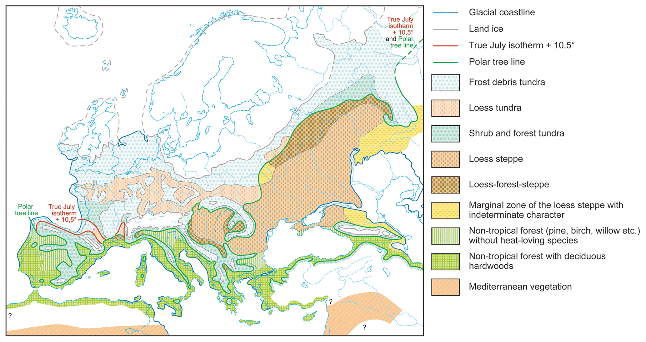
Figure 2The climatic zones of Europe during the Würm glaciation. (1) Ice-age coasts (serration towards the water). (2) Land ice (serration towards the ice). (3) True July isotherm +10.5^∘. (4) Polar tree line. (5) Frost debris tundra. (6) Loess tundra. (7) Shrub and forest tundra. (8) Loess steppe. (9) Loess-forest steppe. (10) Marginal zones of loess steppe of indefinite character. (11) Non-tropical forest (pine, birch, willow and the like) without thermophilic species. (12) Non-tropical forest with more demanding deciduous hardwoods. (13) Mediterranean vegetation.

On the Iberian Atlantic coast, the forest probably did not advance northwards beyond Cape Finisterre under these primitive conditions². On the other hand, the forest on the warm Iberian Mediterranean coast reached much further north. It also encompassed today's Mediterranean France, the Languedoc and Provence (see footnote 1) and here, at the southern foot of the central plateau and the Provencal Alps, it already penetrated close to the +10.5^∘ July isotherm derived from the snow line depression above. Likewise, the investigations carried out further east, at the northern and southern foot of the Alps, in Moravia and Hungary, in Wallachia and especially in Eastern Europe between the Dnieper and the Urals, show that the polar tree line of the Würm glaciation, obtained by pollen analysis, coincides almost exactly with the isothermal line mentioned above³. Thus, there is an extraordinarily good agreement between results obtained in very different ways.

On the Atlantic coast, the polar tree line of the Würm glaciation determined in this way remains about 1000 km away from the nearest point of the Nordic inland ice masses, while in the upper Volga region the ice line and tree line almost touch. This is a sign that it was not a secondary cooling effect originating from the glacial ice that determined the position of the polar tree line at that time, but that both phenomena, the depressions of the snow line (i.e., the expansion of the inland ice) as well as the southward shift of the polar tree line, were dependent on an overriding primary climatic effect. Since the depression of the snow line, but never the shift of the tree line, could be achieved by an increase in winter precipitation, this is further proof that the primary climatic effect causing the glacial periods was in fact a cooling process, primarily of the summer temperatures. This did not occur to the same extent on the whole earth, but in the same direction. In contrast, the precipitation during the ice age did not behave uniformly in the individual climate zones: it may have been partly greater, partly less than today.

Further evidence for the glacial climate is provided by the relationship of the then polar tree line to the distribution of loess in Europe. Using new morphological, stratigraphic and – especially Russian – palaeobotanical material, a strict distinction was made between loess-origin and loess-deposition areas according to their climatic-morphological characteristics. In addition to the river valleys and moraine areas of the time, Dücker (1937) considers all frost debris tundras (Büdel, 1948), which were characterised by strong cryoturbation (i.e., constant processing of fine material into loess-like grain sizes) and of which there was no shortage in Europe at that time, to be loess-origin areas. In contrast, areas of loess deposition could only have been densely overgrown, steppe-like dry grasslands and herbaceous vegetation with no or only very loose tall tree growth, but at the same time only weak frost soil movements. The large European loess area, which begins at the eastern border of the continent between the Caucasus and the Mid Urals with a broad base and then narrows in a wedge-shape westwards to its tip in northern France and Brittany, thus corresponded to a uniform steppe-like vegetation belt. This loess wedge was crossed in its central part, on the route Wiener Pforte – upper Dnieper, by the polar tree line derived above. Towards the pole (in this case north-west) of this line, tree growth was absent due to low summer temperatures; towards the equator (i.e., south-east of this line), tree growth receded to a large extent due to too little precipitation, especially in summer. The part of the large loess wedge situated poleward of the tree line was called “loess tundra”, the part equatorward of it “loess steppe” (see Fig. 2). Regardless of the somewhat richer floristic and faunistic features of the loess steppe, both zones must have been very similar in their overall vegetation character and especially in their climatic-morphological features.

Thus, the steppe wedge extending from Asia to Europe, the western tip of which can today be found in Podolia, Wallachia and at most in the edaphically conditioned small steppe islands of the Alföld, was at that time enormously extended to the north and west. In Brittany it reached as far as the Atlantic coast and lay here (i.e., west of the Wiener Pforte Gate – Upper Dnieper line) poleward of the tree line. West of the Wiener Pforte, the tree line coincided with the tree line in Europe at that time. East of the Wiener Pforte, however, there was a wide gap between the two: the tree line rose far to the north with the great inner-continental summer warmth up to about the 57^∘, while the forest remained deep in the south, approximately in the area of today's Mediterranean vegetation, due to the lack of precipitation in this region. Between the two lines, in the Danube countries and in the whole of southern and central Russia, lay the large area of the loess steppe. According to Gritschuk​​​​​​​'s (1946​​​​​​​) pollen analyses, the sparse tree growth locally present in this area experienced a slight densification at its outermost, somewhat wetter northern edge (in the immediate vicinity of the tree line derived above) to form the “forest steppe”, which then changed beyond the tree line into forest tundra and only then into the pure arctic frost deposit tundra in the immediate forefield of the inland ice. This narrow forest-steppe and forest-tundra fringe on both sides of the tree line, which extended from the upper Dnieper near Chernigov via Moscow and the upper Volga (between Kostroma and the mouth of the Wetluga) to the Mid Urals in the Perm region, was then the only remnant of the boreal forest belt that today separates the southern Russian steppe from the northern Russian tundra in a minimum width of 1100 km (Fig. 2).

West of the Wiener Pforte – Upper Dnieper line, the tree and forest line receded to the southern side of the large loess belt, which thus became the “Loess Tundra”. The northern edge of the loess tundra, which ran from the northern edge of the Podolian plate over the Carpathian foothills and the Central European Börden zone to the Channel coast near Dunkirk and then onto the then dry Channel shelf as far as Brittany, directly abutted the frosty loess tundra, which at that time covered central Poland, central northern Germany and all of north-western Germany, the Netherlands, the dry parts of the North Sea and southern England in a large, closed expanse up to the edge of the inland ice. The northern border of the loess against this zone is known to be mostly very sharply drawn. If it were – according to the previous assumption – a purely dynamic boundary of the outwash from the young-glacial outwash plains and moraines, then it would be difficult to explain its sharpness. Above all, it would then be difficult to understand why the loess cover does not begin immediately outside the ice-marginal valley on the dry high old moraine plateaus of Schleswig-Holstein, northern Lower Saxony and the northern Netherlands. Instead, it begins 100–500 km further south! I therefore see it as a former climatic-morphological boundary. There is no doubt that a lot of loess dust also fell north of this line, but the strong erosion processes prevailing there prevented the formation of closed aeolian sediments in the vegetation-poor frost deposit tundra. How strong these erosion processes in the form of cryoturbation and the formation of frost-solifluction deposits, of scouring and outwash were in fact here, can be clearly seen from the relevant studies by Gripp (1932), Dücker (1933), Florschütz (1938), Lehmann (1948) and especially from the new results by K. Richter contained in this volume. The sharply formed northern boundary of the loess, on the other hand, indicates the equalising line at which, with increasing climatic favour to the south, the formation of a closed carpet of tundra, grass and herbage was possible, in the area of which (at that time as in today's Arctic, cf. Büdel, 1948) a strong reduction of the cryoturbation as well as all other erosion processes took place, so that the deposition of loess blankets became possible here.

That this boundary was indeed climatically conditioned is also evident from the fact that – like any other climate-conditioned polar boundary – it can be traced from there with a gentle rise as a climatic altitudinal boundary in the mountains equatorwards. In the Central Uplands of Germany, this upper loess boundary can be clearly traced in many cases. As is theoretically to be expected, it rises (as do all the other altitude boundaries) from NNW to SSE, from about 300 m in the Weser Uplands to about 600 m at the northern edge of the Alps. It runs roughly parallel to the Ice Age snow line, which rises in the same direction and is only about 800 m higher, thus dividing the space between the Ice Age tree and snow line once again into two different climatic-morphological areas, just as is the case in today's Arctic. In the rougher, higher “frost debris altitudinal zone” of the Ice Age low mountain ranges, very powerful solifluction and strong slope erosion suppressed loess formation. Here we find fossil periglacial cover beds everywhere today (Büdel, 1944), whereas in the depths of the basin landscapes, there are mighty loess deposits without any intercalation of coarser material. Here, in the deeper, densely vegetated “tundra stage” of glacial Central Europe, a closed plant cover prevented stronger frost soil movements and thus made loess deposition possible. In between, there was a struggle zone at medium altitude, where loess on the one hand, solifluction deposits, alluvial debris and coarse blown sand material on the other hand entered into alternating bedding (and indeed into a very typical form of alternating bedding, which will concern us further below). The upper loess boundary is therefore at the same time the lower boundary of strong solifluction phenomena.

Further equatorwards, the dry loess tundra on the humid western edge of Europe changed into a – loess-free – forest tundra, as it probably occupied central France between the Loire and the Garonne, until finally, in the area of today's French Mediterranean region, the polar tree line was also reached here. During the Ice Age, the closed tall deciduous and mixed forest of today's Central European habitus was almost entirely restricted to the Mediterranean countries, which were apparently relatively mild and humid at that time. The space between the polar forest and ice frontiers was thus not only much wider than today's narrow tundra zone at the northern edge of the continent, but also qualitatively quite different and, thanks to the contact between cold and dry steppe, much more extensively structured. By combining all methodological approaches, it is possible to distinguish five large climatic-morphological and phytogeographical zones in the frost debris tundra, forest tundra, loess tundra, loess steppe and loess forest steppe, and to determine their mutual distribution in the main ranges (cf. Fig. 2).

The regularities of loess distribution that become apparent in the process mostly point to a formation by westerly winds. This is also evident from the local depression of the glacial snow line on the western sides of all European mountains and from the fact that, conversely, all the high and late glacial drift sand and dune deposits in Europe are always found only on the eastern side of the sand-supplying glacial valleys. While the loess was also blown up by weaker winds, the drifting sand could only start to move during strong storms. Even in the glacial periods, the strongest winds came from the west, namely when strong storm depressions passed over Europe along the natural migration routes (e.g., along the southern edge of the inland ice, along the northern edge of the Alps and along various routes through the Mediterranean). The distribution of the high and late glacial drifting sand relics clearly shows that the direction of the strongest, morphologically most effective winds in Central Europe must have been the same in many respects as it is today. That is, westerly winds in the Upper Rhine region, in northern Germany and Poland, northerly winds in the northeastern Alföld (Nyirseg) and finally the winds so clearly visible in the dunes and dune valleys of the Danube-Tisza plateau and Pannonia, northwesterly, north-northwesterly and finally – as they approach the eastern edge of the Alps – almost purely northerly wind directions, which radiate almost radially from the Wiener Pforte and which reveal in a particularly clear way the influence of the Alpine mountains on the storm depressions that frequently move towards their northern edge and then turn off towards Hungary (cf. Defant, 1924, especially Maps 7 and 11). It can be assumed that such distinct westerly weather conditions were rarer during the Ice Age, while easterly conditions with high-pressure weather and (mostly weak!) easterly winds were more frequent – especially in winter – than today. It is important to note, however, that the overall mechanism of weather patterns was apparently the same then as it is now. Even if westerly winds blew somewhat less frequently in Central Europe, they were nevertheless the sole bringers of snow, they moved the mass of drifting sand and even in the Late Glacial period shaped the inland dunes to their present form. Only the drifting of the light loess dust was also caused by the (drier, see Klute, 1949) easterly and northerly winds.

This result is consistent with the fact that above we found the course of the Ice Age polar tree line (and also of the loess line) completely unaffected by secondary climatic effects of the inland ice. Obviously, the prevailing planetary westerly winds drowned out such local influences. They probably blew over the former ice sheet in a similar way as today's migrating minima often enough reach over the Greenland ice sheet and wash away its cold air layer, which is always very thin and flows off to the edges, but never becomes weather-effective in the wider area (Loewe, 1935; Georgi, 1939). Finally, the results obtained by Dücker (1933) and others on the distribution of frost soils during the Ice Age show even more clearly that the Ice Age climate was independent of the ice. Frost soils prevailed in the old morainic areas of the entire frost debris periglacial zone during the advance and during the peak of the last glaciation. However, with the passing of the peak, the frost soil effects recede strongly. Traces of strong frost effects can be found in various places under the young glacial deposits, but only sparsely on the young morainic areas, although the ice sheet did not completely disintegrate immediately after the first retreat from the Brandenburg stage, but still had a long hold in the Frankfurt and Pomeranian stages, during which it still had the same size and shape as before. From this finding, Troll (1948) rightly concluded that the climatic change from the High Ice Age to the Late Glacial occurred very suddenly at or even before the ice reached its peak. The ice had already created the frost-soil climate and did not begin to do so. A primary cooling of the atmosphere was the overriding process on which all the phenomena of the Ice Age and the entire shift of the climate belt, including the enlargement of the glaciers, depended. Vegetation, water balance, soil and formative processes reacted immediately to the climatic change that occurred at the end of each glacial period to the following interglacial period. In a fairly short time, the smaller glacier areas also adjusted to the warmer climate with a corresponding decline. The large inland ice masses reacted with much greater delay: they sometimes even reached the peak of their expansion only when the climatic peak of the glacial period had already passed. Nevertheless, the North Polar inland ice masses – of which the Greenlandic land ice is a preserved remnant – still grew during the glacial periods and disappeared during the interglacial periods. In contrast, the Antarctic ice sheet, which even today lies almost entirely above the snow line, seems to have behaved even more extremely: according to Meinardus (1925, 1928)⁴, the glacial periods (with, in my opinion, reduced atmospheric circulation!) were unable to provide it with any additional nourishment, so that it finally grew during the interglacial periods. If one assumes that these interglacial periods correspond to the northern hemispheric interglacial periods, the Antarctic inland ice is delayed to such an extent that its fluctuations are the reverse of the Pleistocene interglacial and glacial periods in the rest of the world.

If, of all the effects of the glacial temperature increase, the inland ice reacted most inertly, then even with its fluctuations it cannot provide an absolute standard for the subdivision of the glacial periods into individual sections. So far, it has been used exclusively as such a yardstick with its phases of advance and retreat and has proved to be very suitable for a stratigraphic subdivision of the glacial period deposits formed in the area of influence of the ice. But the question is how far its phases really correspond to the purely climatic phases of the glacial periods. We will have to look for other, absolute climate scales here. From the pollen analysis, a subdivision of the glacial periods into individual climatic phases (according to the well-known very detailed climatic subdivision of the postglacial period and the last two interglacial periods, cf. the essays by Woldstedt, Firbas, Rein and Selle in this volume) has not yet been possible. After all, there are other ways to go about it. For example, at the above-mentioned loess upper boundary, where solifluction deposits or alluvial sands and loess occur in alternating layers, a very peculiar, always constant relationship between these two fossil soil elements can be observed. In such profiles, there is never an even interlocking from top to bottom. Rather, at the base of such a sequence of layers, which belong together in time, there is always the solifluction deposits, followed by an intermediate zone in which thin horizontal loess layers alternate with solifluction deposit bands or individual (windblown or washed away) sand layers, above which there is often still horizontally layered loess and only then, in the uppermost part of the profile, the actual normal loess with a vertical structure. However, there are also profiles in which the basal solifluction deposits are directly overlain by an initially horizontally stratified loess and then, towards the top, by increasingly pure and vertically fissured loess, with a sharp transition and without the interposition of an intermediary alternating stratification zone. ⁵

If, as in the profiles described by Schönhals in this volume, several loesses of different ages are found on top of each other, then here, too, there are always embedded solifluction deposit layers at the base of each loess layer, followed immediately above by the loess and only on this did the weathered soil of the next interglacial develop. Above this weathering layer, the basal solifluction deposits of the next glacial period follow. That such a loess was once directly overlaid (i.e., without an intermediate weathering horizon) by a solifluction deposit from the same glacial period has never been observed so far! As far as layers of this type are alternating, each glacial period regularly begins with a solifluction deposit and ends with a loess! A generous regularity is recognisable here. It can only be interpreted in such a way that each “Ice Age” is divided climatically into two periods: a first, perhaps cooler in summer, but certainly wetter, more oceanic in character, in which solifluction deposits also dominated the deeper regions of Central Europe and the conditions for loess formation (dryness and dense, steppe-like vegetation) were unfavourable. Then followed the drier loess period with strong wind effects and at the same time perhaps a slight upward movement of the steppe-like vegetation of the loess tundra, i.e., probably on the whole a more continental climate impact. The first cooler, humid period of the Early Glacial would then be the time of the growth of the large inland ice masses, the second drier period that of their peak (Late Glacial), which would then be followed by a third, warmer and more humid Late Glacial, i.e., essentially the time of the melting of the glaciers.

The formation of the non-glacial Würm glacial valleys shows a similar multiphase pattern. Their broad valley bottoms, formed by the transport of the greatly enlarged ice-age debris masses, whose always slightly arched cross-section proves their formation by a uniform large-scale filling process (Büdel, 1944), can be divided everywhere into two low terrace levels according to the investigations carried out in the uplands of Lower Saxony by my student H. Mensching. One, which is older and wider, forms the morphologically well-developed “upper Lower Terrace” about eight to ten metres above today's river level and is only reached in places even by the highest floods. The second is a deeper and narrower one, which as the “lower Lower Terrace” tends to lie only 3–5 m above the river level, which is still regularly reached by floods. Therefore, its basal glacial gravel body is usually covered by a subsequent Holocene alluvial loam layer. Climatically, both Lower Terraces must have originated from different phases of the last ice age. Since the “upper Lower Terrace” is also always completely loess-free, it must be younger than the Early Glacial solifluction deposit Period. It therefore probably corresponds to the High Glacial loess Period itself, while the lower Lower Terrace probably belongs to the Late Glacial. This is also supported by the fact that the lower Lower Terrace is limited to the main valleys and the larger side valleys. It is absent in the higher side valleys and thus obviously did not have the time to reach back into the last branches of the river courses to form the valley floor before the completely different valley formation processes of the geological present began with the onset of the post-glacial period. This is why in our low mountain ranges the valley bottoms of the uppermost valley branches often “hang” above those of the larger valleys; in some cases, such “fluviatile step mouths” are 15 m high! Of the Würm glacial valley forms still preserved today, only the first formation of the trough-shaped uppermost valley beginnings (corrosion valleys, depressions) apparently goes back to the early glacial solifluction deposit period, because these are always present on the flanks of larger valleys only above the “upper Lower Terrace” and the solifluction deposit streams that can occasionally be detected in them are sometimes still loess-covered, i.e., they were already no longer moved during the high glacial loess period.

A more precise division of the Würm glaciation into individual climatic phases has meanwhile been made elsewhere (Büdel, 1950).

In the preceding, it is to be demonstrated first and foremost that a much stronger spatial differentiation of the Ice Age climatic zones can be carried out by the combined evaluation of all climate evidence that can be used and that the same method also allows a temporal classification of the Würm glaciation independent of the delayed development of the inland ice masses.